Linear Elastic Lateral Buckling (Including Shear Deformation) and Linear Elastic Lateral Torsional Buckling of Composite Beams - an Analytical Engineering Approach- Juniper Publishers

Juniper Publishers- Journal of Civil Engineering

Abstract

This article outlines a concise and complete versatile novel analytical framework to quickly and effectively assess lateral shear (knik) and lateral torsional buckling (kip) of composite beams build of sections with different lengths. The adjective "composite” includes dissimilar beam cross-sections (beam profiles) and distinct beam materials. The major aim is to provide engineers with an accurate, simple but elegant, practically applicable and analytical beam buckling tool based on advanced solid theoretical propositions or background. The justification of the analytical theory is supplied by demonstration of executed numerical tests (i.e. finite element method), which affirm the validity of the proposed analytical buckling models adapted to the considered beam buckling cases.

Keywords: Lateral buckling; Lateral torsional buckling; Composite beam; Analytical formulation; Shear deformation; Linear elasticity

Introduction

Buckling means the loss of stability of an equilibrium configuration of a structure. Elastic buckling is a state at which the structure loses its stability and large elastic deflections will start developing rapidly. It is normally associated with the minimum eigen value of the perfect structure, i.e. often referred to as classical buckling [1]. In this article attention is confined to linear elastic composite beam buckling (especially lateral and lateral torsional buckling phenomena). An abbreviated and lucid literature survey and comprehensive discussion about lateral and lateral torsional buckling of structural members is rendered in the dissertation of Raven [2] and the article of Vander Put [3]. It should be highlighted that the adjective "composite” refers to multiple beam cross-sections and beam materials.

Approximate solution methods are frequently encountered and used in engineering design practice for tackling beam buckling problems. In particular, summation theorems (i.e. Foppl Papkovich theorem) are appropriate and advantageous because of their robustness, accuracy, easiness and algebraic simplicity [4]. It should be kept in mind that there is similarity or analogy with parallel and serial analytical approaches of spring systems, electric systems or hydraulic systems (the so-called analogies).

The key goal of this article is to address respectively formulate an effective analytical tool for reliable (engineering) estimation or approximation of the linear elastic lateral shear buckling force and linear elastic lateral torsional buckling moment of composite beams made of non-overlapping parts based on the indicated summation theorem and corresponding well-established structural elastic stability notions [5]. A succinct but detailed exposition of the previous stated matters and issues is offered in the subsequent sections.

Preliminaries and Requisites

Global Cartesian ( components) and local Cartesian ( components) right-handed coordinate systems are used. The former identify the composite beam orientation, beam location and beam external loads, while the latter define attached geometrical (shape and size) properties of the homogenous beam cross-sections. It is henceforth assumed that the origin of the local coordinate system is located at the centroid C of the cross-sectional area. In addition, the initial (undeformed) geometry of the composite beam is a straight line. 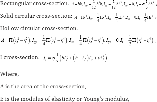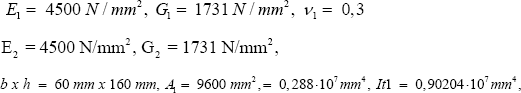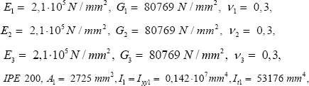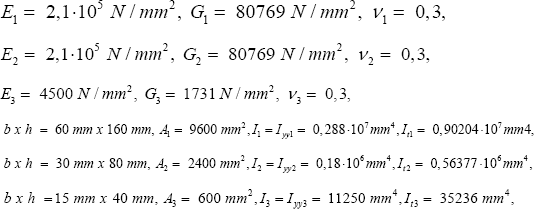The following beams cross sectional quantities (properties) are employed [6].

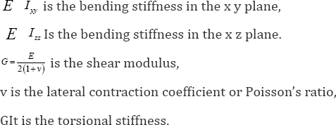
Where,

A is the cross sectional area,

I_yy , I_yz , I_zy and I_zz are called second moments of area.

Where, I_t is the torsion constant.

Note 1: The centroid C is defined as that point of an area A for which the static moments of area are zero when the origin of the local xyz coordinate system is chosen there, i.e.

The normal centre NC is specified as that point of the crosssectional area where the resultant of all normal stresses due to extension has its point of application.

Note 2: In a homogenous (single material) cross-section, the centroid C and normal centre NC coincide.

Note 3: The adopted assumption I _yz = I_zy = 0 implies that the selected beam cross section has at least two lines of symmetry.

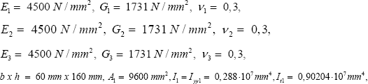
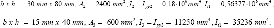
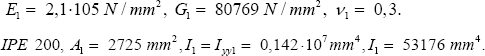
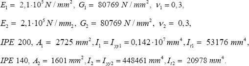
Note 4: I _yy and I_zz are commonly indicated as the moments of inertia and I _yz , I _zy are known as the product of inertia. The Equations (1) have been applied to the cross-sections in Figure 1. The results are Shown below.

Linear elastic lateral buckling (including shear deformation) (knik)

Model geometry

The typical model geometry is depicted in Figure 2. The following mechanical boundary (displacement and load) conditions are implemented (prescribed).

Boundary 1: u_X = O, u_Y = O, u_z = O , F_x = l (applied at centroid)

Boundary 2: u_Y = 0, u_Z = 0 , F_X = -1 (applied at centroid)

Note 1: A set of balanced forces is obligatory in order to preserve equilibrium of the composite beam in the analytical model configuration.

Note 2: The prescribed boundary displacement constraints prevent rigid body motions (circumvent singularities in the numerical (finite element) solution process).

Analytical model

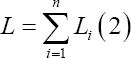
The composite beam with length L is made of segments i with corresponding length L_i (Figure 3) and each segment (section) i has the accompanying attributes Young's modulus E_i shear modulus G_i , shear deformation coefficient k_si [7,8] crosssection area A_i and second moment of area I_i Furthermore, the cross-section of each segment i fulfils the condition I_yyi < I_zzi , which implies that I_i=I_yyi Consequently, the following relation holds.

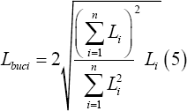
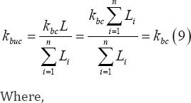
The engineering estimate of the buckling length L_tmci segment i is given by the expression

L_buci = k_bucL_i (3)

Where,

K_buc Is the buckling length factor, which is identical for each segment in the particular composite beam arrangement.

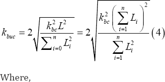
K_bc Is the buckling length factor of the composite beam, dependent on the mechanical boundary conditions (supports). In this specific case of a composite beam with span L and supported by two hinges at the edges k _bc = 1.

It is emphasized that the buckling length of the composite beam depends only on the boundary conditions and thus not on cross-sectional properties. Substitution of Equation 4 into Equation 3 produces the following identity.

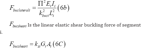
Subsequently, the linear elastic lateral shear buckling force F_buci of segment i is universally elaborated as shown in Equation 6a. Note that shear deformation is also incorporated, see [5], (Timoshenko 1985).

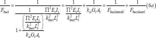
F_buc Is the linear elastic lateral shear buckling force of segment i,

F_buclaterali Is the linear elastic lateral buckling force of segment i,

Recalling from literature that the Foppl-Papkovich theorem (Tarnai 1995) is valid for this case, the following lateral shear buckling system force equation is stated in general format.

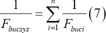
F_bucsys Is the linear elastic lateral shear buckling force of the composite beam (also denoted as system), n Is the total number of considered segments.

The aforementioned formulae devise the complete linear elastic lateral shear buckling analytical model.

Numerical verification (case studies) knik

Three case studies (KNIK 1, KNIK 2 and KNIK 3) are conducted and concisely presented in order to examine the validity and soundness of the proposed analytical approach by comparison with numerical results obtained by the finite element method [9,10].

Case study KNIK 1-1

Case KNIK 1-1 considers a wooden beam of one segment (Figure 4).

The properties are L = 3000 mm, L1 = 3000 mm, K_buc = 1,K_bc = 1,F_X=±N,

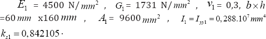
The obtained results are F_{bucsysnumerical} =14214N and F_{bucsysnumerical} = 14221N (Figure 5).

Case study KNIK 1-2

Case KNIK 1-2 considers a composite wooden beam of two segments (Figure 6).

The results are F_{bucsysamlytical} =I673N, F_{bucsysnumerical}= I443N (Figure 7). The deviation is -13, 74 %.

Case study KNIK 1-3

Case KNIK 1-3 considers a composite wooden beam of three segments (Figure 8).

The properties are L = 3000 mm, L1 = 1000 mm, L2 = 1000 mm, L3 = 1000 mm,

The results are F_{bucsysanalytical} =156 N and F_{bucsysnumerical} = 161 N (Figure 9). The deviation is +3, 11 %.

Case Study KNIK 2-1

Case KNIK 2-1 considers a steel beam of one segment (Figure 10).

The properties are L = 3000 mm, L1 = 3000 mm, K_buc = 1,K_bc = 1,FX=±N,

The obtained results are F_{bucsysnumerical} =328263N and F_{bucsysnumerical} = 326493N (Figure 11).

The deviation is -0,539 %.

Case Study KNIK 2-2

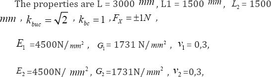
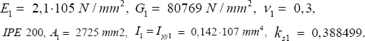
Case KNIK 2-2 considers a composite steel beam of two segments (Figure 12).

The properties are L = 3000 mm, L1 = 1500 mm, L2 = 1500 mm, k_buc = 2, k_bC = 1, FX = ±1 N,

The results are F_{bucsysnumerical} = 157757N and F_{bucsysnumerical}= 147745N (Figure 13) the deviation is -6,346%.

Case Study KNIK 2-3

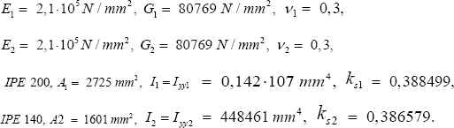
Case KNIK 2-3 considers a composite steel beam of 3 segments (Figure 14).

The properties are L = 3000 mm, L1 = 1000 mm, L2 = 1000 mm, L3 = 1000 mm,

The results are F_{bucsysanalytical} = 47024N and f_{bucsysnumerical}= 48983N (Figure 15). The deviation is +4,165 %.

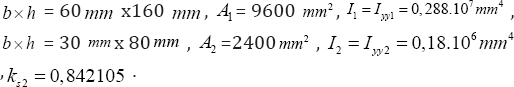
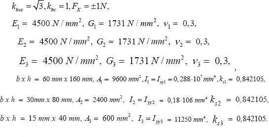
Case Study KNIK 3-3

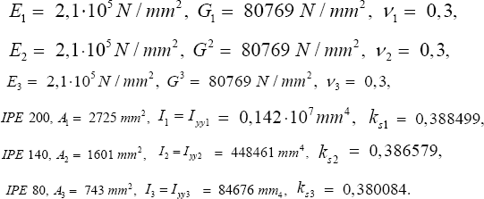
Case KNIK 3-3 considers a composite steel-wood beam of three segments (Figure 16).

The properties are L = 3000 mm, L1 = 1000 mm, L2 = 1000mm,L3 = 1000 mm,

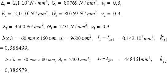
The results are = 166 N and = 171 N (Figure 17). The deviation is +3,012 %.

Linear elastic lateral torsional buckling (kip)

Model geometry

The governing model geometry is shown in Figure 18. The following mechanical boundary (displacement and load) conditions are implemented (prescribed).

Boundary 1: u_x = ^{0 u_y = 0 u_z = 0 , φ_x = 0, M_z = -1 (applied at centroid).}

Boundary 2: u_y = 0 u_z = 0 , φ_x = 0,

M_z = +1 (applied at centroid).

Analytical model

The model for lateral torsional buckling is mostly identical to the models for lateral buckling (Section 7.2). Not used in lateral torsional buckling is the shear deformation coefficient k_s1. Extra is the is the torsional constant I_ti,. The cross-sectional warping stiffness of segment i is assumed to be negligible. The engineering estimate of the buckling length L_buci of segment i is

L_buci = k_bucL_i (8)

Where,

k_buc Is the buckling length factor. Which, is the same for each segment in the specific composite beam configuration

k_buc Is the buckling length factor of the composite beam, dependent on the mechanical boundary conditions (support). In this specific case of a composite beam with span L and supported by two forks at the edges:

k_bc = 1

It is underlined that the buckling length of the composite beam is only dependent on the boundary conditions and hence not on cross-sectional properties. Substitution of Equation 9 in Equation 8 produces the following identity.

L_buci = k_bucL_i (10)

Taking into account the previous settled propositions, the linear elastic lateral torsional buckling moment M_buci of segment i is

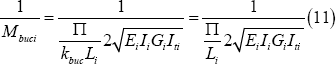
The Föppl-Papkovich theorem (Tarnai 1995) is apt for this case. The following lateral torsional buckling system moment equation is written in universal layout.

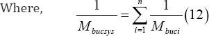
M_bucsys Is the linear elastic lateral torsional buckling moment of the composite beam (also symbolized as system).

n is the total number of segments.

The aforesaid procedure details the full linear elastic lateral torsional buckling analytical model.

Numerical verification (case studies) kip

Three case studies (KIP 1, KIP 2 and KIP 3) are consecutively undertaken and compendiously offered in order to inspect the legality or reliability of the analytical approach by judgment of numerical results.

Case study KIP 1-1

Case KIP 1-1 considers a wooden beam of one segment (Figure 19).

The properties are L = 3000 mm, L1 = 3000 mm, k_buc = 1, k_bc =±1 Nmm,

The results are M _{buaysanaiytcai} = 0,149-108 Nmm and M _{buaysanaiytcai}= 0,149-108 Nmm (Figure 20).

Case study KIP 1-2

Case KIP 1-2 considers a composite wooden beam of two segments (Figure 21).

The properties are L = 3000 mm, L1 = 1500 mm, L2 = 1500 mm, k_buc = 1, k_bc = 1, MZ = ±1 Nmm,

The results are M _{buaysanaiytcai} = 0,175-107NmmM _{buaysanaiytcai} and =0,176-107Nmm (Figure 22).

The deviation is +0, 57%.

Case study KIP 1-3

Case KIP 2-3 considers a composite wooden beam of three segments (Figure 23).

The properties are L = 3000 mm, L1 = 1000 mm, L2 = 1000 mm, L3 = 1000 mm, k_buc =1, k_bc = 1, M_z = ±1 Nmm,

The results are M _{bucsysanalytical} = 163701 Nmm and M_{bucsysnumerical} = 164801 Nmm (Figure 24).

The deviation is +0, 67 %.

Case study KIP 2-1

Case KIP 2-1 considers a steel beam of one segment (Figure 25).

The properties are L = 3000 mm, L1 = 3000 mm, k_buc = 1, k_bc = 1, —_z = ±1 Nmm,

The obtained results are M _{bucsysanalytical} = 37, 48-106 Nmm and M _{bucsysanalytical} = 37,5-106 Nmm (Figure 26).

The deviation is +0,053 %.

Case study KIP 2-2

Case KIP 2-2 considers a composite steel beam of two segments (Figure 27).

The properties are L = 3000 mm, L1 = 1500 mm, L2 = 1500 mm, k_buc = 1, k_bc = 1, MZ = ±1 Nmm,

The results are M _{bucsysanalytical} = 19, 55-106 Nmm and M _{bucsysanalytical}= 19, 2106 Nmm (Figure 28).

The deviation is -1, 79 %.

Case study KIP 2-3

Case KIP 2-3 considers a composite steel beam of three segments (Figure 29).

The properties are L = 3000 mm, L1 = 1000 mm, L2 = 1000 mm, L3 = 1000 mm, k_buc = 1, K_c = 1, MZ = ±1 Nmm,

The results are = 6, 91-106 Nmm are = 6, 68-106 Nmm (Figure 30).

The deviation is -3,328 %.

Case study KIP 3-3

Case KIP 3-3 considers a composite steel-wood beam of three segments (Figure 31).

The properties are L = 3000 mm, L1 = 1000 mm, L2 = 1000 mm, L3 = 1000 mm, k_buc = 1, k_buc = 1, MZ = ±1 Nmm,

The results are = 174324 Nmm and = 175756 Nmm (Figure 32).

The deviation is +0,821 %.

Conclusion

Numerical evaluation confirms the correctness of the presented linear elastic lateral shear and lateral torsional buckling analytical models. The deviations between the analytical and numerical approach are rather small and reveal clearly the ability to yield realistic outcomes. The supplied analytical linear elastic buckling models produce accurate and reliable values, which can be classified as suitable for engineering design purposes. Needless to cite that the analytical approach should always be cautiously applied and the results ought to be methodically checked by the responsible structural engineer. A salient observation is that the presented tactic could also be invoked for linear elastic buckling assessment of castellated and cellular (steel) beams. However, this assertion has not yet been verified and is thus speculative. Insertion of plasticity is straightforward however treatment of this topic is beyond the scope of this article.

For More Open Access Journals Please Click on: Juniper Publishers
Fore More Articles Please Visit: Civil Engineering Research Journal