New Approach to Obtain an Optimal Value for MQ-RBF Shape Parameter for the Nonlinear Analysis of Elastic Thin Plate- Juniper Publishers

 Civil Engineering Research Journal- Juniper Publishers

 

Abstract

A new approach in using a multi-quadric radial basis function (MQ-RBF) in the analysis of nonlinear behaviour of elastic thin plate is provided. The approach provides a new method to obtain an optimal value of the shape parameter, c, involved in the (MQ-RBF). The shape parameter c plays a very important role in the accuracy and stability of the solution. The approach uses approximate exact linear solutions of linear analysis of the thin plates as standpoint toward the calculation of the optimal c value. Then, the optimal c values were implemented in the analysis of nonlinear thin plate behaviour. Combinations of different boundary conditions (simply, and clamped), for a square thin plate under uniform distribution loads were analysed. The accuracy of the adopted approach has been validated by comparing the results with FEM solutions. The comparison shows that the approach can be used effectively in obtaining the optimal value of c.

Keywords: Thin plate; MQRBF; Nonlinear analysis; Shape parameter; Finite element method; Boundary element method

Introduction

The analysis of the elastic thin plate under different loads with various boundary conditions is provided by two main theories (small and large deflection) [1,2]. In the small deflection theory, linear analysis is adopted. For such cases, approximate exact solutions for different boundary conditions, loads and shapes are available like the ones in Timoshenko book [1]. However, the nonlinear behaviour analysis is adopted by the large deflection theory [1]. The nonlinearity comes from the coupling of the three governing partial differential equations as described in [1,2] for the transverse and lateral deformations. Some attempts to find approximate exact analytical and semi-analytical solutions for some cases of the large deflection analysis are provided [3-5]. However, several assumptions and restrictions were employed in order to have such solutions which make those attempts very limited and not valid to cover wide range of variation of real problems. On the other hand, and to handle numerous real problems, numerical solutions were adopted. Numerous numerical methods are available such as finite element method (FEM), boundary element method (BEM), finite difference method (FDM), etc [6-12]. The most common numerical method is the FEM which has been approved as a very good method in terms of the accuracy and flexibility. However, and despite of the intensive research in FEM, there are still some problems raised such as the ones because of the distortion from the large deflection which needs re-meshing during the analysis.

To overcome the re-meshing generation problems, different researchers have adopted meshless or mesh-free numerical methods in the last decades [13-29]. Several types of such methods are adopted to solve different problems. According to the literature, the MQ-RBF based meshless method is the best method that can handle the solution of the partial differential equation applications. However, the shape parameter, c, involved in the MQ-RBF plays a very important role in the accuracy and stability of the solution. The main concern is the determination an optimal value of c [13-15]. From the literature, several approaches and attempts to get optimal values of c are provided [13,28-34]. Those approaches depend mainly on the available data for which MQ-RBF is used as an interpolant. In this paper, a different approach is adopted to get the optimal value of c using the linear exact solution of the thin plates. The description of the method is provided in section 2. The method has been tested using several examples such as simply, clamped, and simply clamped square plate under uniform distribution loads. The results show that the adopted method is an effective tool to get the optimal value of c.

Method Description

The method of finding an optimal c value using exact linear solution for elastic thin plate is summarized as follows:

1) Implement the exact solution and get the deflection function, w.

2) Divide the plate to specific number of nodes (in the domain and in the boundary).

2) Divide the plate to specific number of nodes (in the domain and in the boundary).

4) Represent w by MQ-RBF as it is shown in Section 3.

5) Assume initial value for c, let it equal to the minimum distance between the nodes.

6) Apply the governing partial differential equation for the transverse deflection, w which is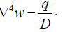 

7) Apply the boundary conditions according to the specified problem

8) Solve the developed equations in the steps (6) and (7) to get the required coefficients in step (4)

9) Calculate the difference between the obtained deflections in step (4) and step (3).

10) Change the value of c with a specific scheme and repeat steps from 6 to 9

11) Repeat step 10 for several values of c and then take the optimal c values which make the calculated difference in step 9 within 5%.

Formulation of the Problem

Governing Equations and Boundary Conditions

For an elastic thin plate undergoing large deformation, the governing equilibrium equations are expressed in terms of the out of plane deformation, w and the in-plane deformation u and v. Here is the summary of the formulations and their boundary conditions as follows [28, 29];

Subscript variables in the previous equations represent partial differentiation with respect to the variables.

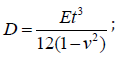
t is plate thickness, ν is poisson’ s ratio, E is Young’s Modulus and q is uniform load

A. Boundary Conditions

Two main types of boundary conditions can be categorized for large deformation of thin plates. The out-of-plane boundary conditions are found in both small and large deflection theories whereas the in-plane boundary conditions are found only in the large deformation theory.

a. For the in-plane boundary conditions, u = v = 0.

b. For the out-of-plane boundary conditions, there are two primary boundary conditions at each point in the boundary as follows:

Regarding the shear, Vn, it was divided into two components

where 𝑛𝑥 and 𝑛𝑦 represent the unit vector components normal to the boundary, 𝑥 and 𝑦 respectively.

RBF Formulations

The nature and definition of RBF depends on the radial distances between the points. For 2-Dimensional problem like the one in this study, x and y axes are considered. For general body shape, it is divided into two main parts, the domain (Ω) and the boundary (Γ). Both the domain and the boundary are divided into several points (xD, yD) and (xB, yB) respectively as shown in Figure 1.

The number of points in the domain and boundary denoted by ND and NB respectively. The total points Np = ND + NB . MQ-RBF is defined as: where c is the shape variable or parameter.

To solve the thin plate problem using MQ-RBF, the out of plane deformation, w, and the in-plane deformations, u and v, are represented by a combination of MQ-RBF with constants as described below.

Where, are constants and can be determined by applying the governing equations and boundary conditions. For the purpose of programing the solution, the governing equations as well as the boundary conditions for both out and in-plane deformations are summarized and organized in matrices forms as follows:

The out of plane matrices;

They are denoted by: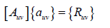 

They are denoted by: 

The procedure of the solution of equations (4) and (5) is as follows:

1. Input data such as geometry, boundary conditions, materials, loads, the optimal c value calculated in section 2 above.

2. Calculate Aw and Auv

3. Calculate the inverses of Aw and Auv

4. Apply load increment

5. Initialize the nonlinear terms (NL1(w), NL2(w), VNL, and NL3(w,u,v))

6. Calculate aw and auv

7. Get w, u, and v

8. Calculate w at the centroid of the plate

9. Evaluate the nonlinear terms, mentioned in Step 4

10. Repeat steps 6 to 8

11. Calculating the error which is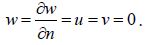 

12. If the error is < 0.05%, go to Step 4 to apply the new increment and repeat the steps from 5 to 12 until the whole load is applied.

13. If the error is not less than 0.05%, repeat steps from 9 to 12.

Numerical Examples

General information has been used for all examples. The material dimensionless properties are the same, which are as follows: Young’s modulus E=10000, Poisson’s Ratio ν=0.3. The plate thickness is t=0.1. Uniform node distribution has been adopted for all as it is shown in the Figure 2 below.

In addition, the results of the solutions (exact, MQ-RBF for linear analysis, MQ-RBF for Nonlinear analysis, and Finite Element Analysis for nonlinear analysis), are shown in tables and charts. For the linear analyses, the results include optimal c values, deflections, w, from exact and MQRBF solutions at the centroid of the plates. Comparisons between the corresponding solution results are shown as well by calculating the differences. However, for the nonlinear analyses, the deflection, the bending and membrane stresses results for both the MQRBF and FEM solutions in tables and charts. In addition, the differences between the MQ-RBF and FEM solutions are provided for validation.

Clamped–Clamped Supported Square Plate (CCS)

A square plate with dimensions a=b and clamped supports on all sides, is analysed under dimensionless uniform load, q=160. The exact solution for the nonlinear analysis is given by Timoshenko & Woinowsky-Kreiger [1]. (Figure 3)

The results of the analysis using the exact solution and the MQ-RBF for the deflections at the centre of the plate for q=60 are given in Table 1. The results contain the exact, MQ-RBF, differences as percent and the corresponding c values. From the results shown in Table 1, the optimal c values are 0.2 and 0.8.

The optimal c values obtained from Table 1 are used in the large deflection analysis for the plate. The total load, q = 160, has been applied incrementally with load increment of 20. The dimensionless results of deflection, bending stresses, and membrane stresses are shown in Table 2 and Figures 4-6. Comparison between the MQ-RBF and FEM is included in Table 2 as differences in percent.

Simply – Simply Supported Square Plate (SSS)

A square plate with dimensions a = b and simple supports on all sides, is analysed under dimensionless uniform load, q = 48. The exact solution for the nonlinear analysis is given by Timoshenko & Woinowsky-Kreiger [1]: (Figure 7)

The boundary conditions are; 0 n w = M = u = v = , on all boundaries.

The results of the analysis using the exact solution and the MQ-RBF for the deflections at the center of the plate for q=18 are given in Table 3. The results contain the exact, MQ-RBF, differences as percent and the corresponding c values. From the results shown in Table 1, the optimal c values are 0.3 to 0.9.

The optimal c values obtained from Table 1 are used in the large deflection analysis for the plate. The total load, q=48, has been applied incrementally with load increment of 6. The dimensionless results of deflection, bending stresses, and membrane stresses are shown in Table 4 and Figures 8-10. Comparison between the MQ-RBF and FEM is included in Table 4 as differences in percent.

Clamped–Simply Supported Square Plate (CSS)

A square plate with dimensions a=b and clamped supports on two sides and simply supports on the other two sides, is analysed under dimensionless uniform load, q=96. The exact solution for the nonlinear analysis is given by Timoshenko & Woinowsky-Kreiger [1] (Figure11)

The boundary conditions are;

On sample support sides 0 n w = M = u = v = and

On clamped supports sides 

The results of the analysis using the exact solution and the MQ-RBF for the deflections at the center of the plate for q=36 are given in Table 5. The results contain the exact, MQ-RBF, differences as percent and the corresponding c values. From the results shown in Table 1, the optimal c values are 0.2 to 0.9.

The optimal c values obtained from Table 1 are used in the large deflection analysis for the plate. The total load, q = 96, has been applied incrementally with load increment of 12. The dimensionless results of deflection, bending stresses, and membrane stresses are shown in Table 6 and Figures 12-14. Comparison between the MQ-RBF and FEM is included in Table 6 as differences in percent.

Results Discussion

As shown in the results in Section 4, one can get several interesting observations. For the clamped supported plate (CCS), from Table1, the minimum difference between the exact solution and the MQ-RBF solution for the deflection at the centre of the plate is 0.627 % at value of c = 0.7. The differences are less than 5 % for the values of c ranging from 0.2 to 0.8. As a result, the large deflection analysis has been done for the plate using several values of c for the mentioned range. In Table 2, the results of the deflection, bending and membrane stresses at the centre of the plate from both FEM and MQ-RBF at c=0.3 and their differences are provided. It has been noticed that, the maximum difference of the deflections is 1.4% and the bending stresses is 3%. However, the maximum difference of the membrane stresses is 5%. In general, the differences are within 5%. From Figures 4-6, it is clear that the results from the MQRBF and FEM are almost the same which means that the differences are so small.

Likewise, the simply supported plate has the same trend. From Table 3, the minimum difference is 0.1686% at c=0.3. Also, the differences are still less than 5% for the c values ranging from 0.2 to 0.9. Using the optimal values of c, the nonlinear analysis for the simply supported plate has been carried out and the results of the deflection, bending and membrane stresses at the centre of the plate from both FEM and MQ-RBF at c=0.6 and their differences are provided in Table 4. It was noticed that, all the differences are within 5%. In addition, the graphs shown in Figures 8-10 show excellent agreement between the FEM and MQRBF solutions. The same observations were noticed from the third example which is the Clamped-Simply supported plate (CSS). All the differences are within 5% for the values of c ranging from 0.2 to 0.9 as shown in Table 5 and shown in Table 6 for the nonlinear analysis at c=0.2. A very good agreement between the MQRBF and FEM solution is satisfied as shown in Figures 12-14.

Conclusion

From this study, it can be concluded that the adopted approach of finding optimal c values from the comparison of the available approximate exact solutions and MQRBF solution for the linear analysis of thin plate has been demonstrated to be an effective tool. The range of the optimal c values are between 0.2 to 0.8, for the three different boundary conditions (clamped (CCS), simply (SSS), and clamped-simply (CSS)), used in the study. The optimal c values were used in the nonlinear analysis of the three examples and then validated by the FEM solutions. A very good agreement between the MQRBF and FEM solutions is observed for the three different examples. Because of the availability of approximate linear exact solutions for most of the engineering problems, the adopted approach can be utilized for other cases easily to obtain optimal c values, which can be used in the analysis of the nonlinear problems with good accuracy.

For more open access journals, please click on: Juniper Publishers
For more civil Engineering articles, please click on Civil Engineering Research Journal

https://juniperpublishers.com/cerj/CERJ.MS.ID.555724.php