An Operational Analysis and Congestion Estimation of Urban Bus Route Based on ITS- Juniper Publishers
Juniper Publishers- Journal of Civil Engineering

Abstract
This study attempts to make use of traffic behaviour
on the aggregate level to estimate congestion on urban arterial and
sub-arterial roads of a city exhibiting heterogeneous traffic conditions
by breaking the route into independent segments and approximating the
traffic flow behaviour of the segments. The expected travel time in
making a trip is modelled against sectional traffic characteristics
(flow and speed) at origin and destination points of road segments, and
roadway and segment traffic characteristics such as diversion routes are
also tried in accounting for travel time. Predicted travel time is then
used along with free flow time to determine the state of congestion on
the segments using a congestion index (CI). A development of this kind
may help in understanding traffic and congestion behaviour practically
using easily accessible inputs, limited only to the nodes, and help in
improving road network planning and management.
Keywords: Congestion; Delay; Origin and destination; Traffic; Travel time
Abbreviations: TTI:
Travel Time Index; CI: Congestion Index; RMSE: Root Mean Squared Error;
ANOVA: Analysis Of Variance; DDF: Denominator Degrees Of Freedom;
NRMSE: Normalized Root Mean Squared Error; MAPE: Mean Absolute
Percentage Error
Introduction
Traffic congestion is one of the most conspicuously
worsening problems associated with traffic engineering and urban
planning, with clear implications on spheres of urban economy,
environment and lifestyle. Traffic in cities continues to grow
meteorically especially in major cities of developing countries, which
are characterized by heavy economic and population growth. This
naturally necessitates intense transportation of goods and passengers,
increasing demand for personal vehicular ownership that over the last
decade has seen exponential growth worldwide. However, the failure of
sufficiently rapid infrastructural development required to cater to this
burgeoning traffic frequently leads to failures of the urban
transportation system, resulting in traffic jams. Quantification of
congestion thus becomes essential in checking congestion in order to
provide a sustainable transportation system that necessitates a
well-functioning well-integrated urban economy.
Objective
The complexity of traffic systems in several
developing countries is exacerbated due to the prevalence of
heterogeneous traffic that only furthers the chaotic nature of the
study. This study aims to understand the relationship between the
traffic conditions of the source and the destination in segments of an
arbitrarily chosen trip on an arterial and sub-arterial road in a major
metropolitan city of India characterizing extremely diverse traffic
condition. For this purpose, the basic traffic parameters, such as
volume, speed, density and capacity are measured or calculated at
different nodes of the study route and tried against the aforementioned
indicator of congestion: Congestion Index, and a review for the prepared
model and the behavior of the variables used is then prepared.
Research Survey
Congestion has been variously defined as a physical
condition in traffic streams involving reduced speeds, restrained
movement, extended delays and paralysis of the traffic network. The
definition of congestion has been conventionally categorized on the
basis of four parameters: capacity, speed, delay/travel time and cost
incurred due to congestion. Speed based measures of congestion are more
efficient in explaining the degree of congestion [1].
Anjaneyulu and Nagaraj developed a methodology of determining the state
of congestion on road segments with the help of coefficient of
variation of speed. Chakrabartty and Gupta in 2015 estimated the cost of
congestion on a route in Kolkata, based on the methodology devised by
R.J. Smeed [2,3].
Congestion can be defined as the travel time or delay incurred in
excess of that in light or free flow conditions. Time based measures
provide a stronger basis for more generalised conclusions and indicators
like Travel Time Index (TTI) and its derivative Congestion Index (CI)
are easy to comprehend [4].
Though several travel time/delay based measures of congestion such as
Travel Time, Travel Time Index, Travel Rate Index, Delay Rate, Delay
Ratio and Buffer Rate Index exist; this study makes use of Congestion
Index (CI) because of its ease of calculation and intensive nature as a
ratio. The use of origin and destination (O-D) based congestion
estimation in theory is limited. Conventionally, O-D matrices are used
for trip planning, traffic management and operation studies [4].
Methodology
The first step was to identify a suitable route that
includes both arterial and sub-arterial roads and is often wrought with
congestion. Subsequently the route was divided into segments and for
this purpose, eight nodes were chosen, most of them being major rapid
transit bus stops or major intersections. The next step was
identification of potential factors. Both roadway as well as traffic
parameters were considered, and the congestion parameter to be modelled
was fixed (Congestion Index, CI). Once the expected data input was
rightly identified, data were collected on site using video camera for
recording node based traffic parameters and moving car method for
measuring the real travel time [5].
The data were pre-processed and source- destination and segment
variables were calculated. Finally, all variables found were tested for
statistical relationships with the dependent variable, CI, in several
combinations using 75% of the observed data. This model was validated
for the remaining 25% observed data with the help of root mean squared
error (RMSE). Free flow time was then calculated for each segment and
congestion index was found using the predicted values of travel time and
free flow time.
Study Route
Delhi is a rapidly growing major city of India that
characterized by heterogeneity of traffic composition and suffers from
aggravating traffic system [6].
The Delhi route chosen for study comprised two sections: a long eastern
part of the Inner Ring Road, an arterial way, and Sri Aurobindo Marg, a
divided sub-arterial that takes diversion from the Ring Road south of
AIIMS. Each portion consists of three segments separated by a total of
eight nodes (points). The total length of the study route is about
27.4km, excluding a 640m long stretch between AIIMS North Gate and AIIMS
West Gate that was not used for observations. Table 1 & 2 include the roadway details of the study route.


Data Collection
Data collection primarily involved traffic parameter observation on study points such as categorized vehicular traffic volume and spot speed using manual counting and radar gun respectively in count periods of 15 minutes, and travel time using the moving car method. The traffic data were collected in six motored vehicular categories: standard cars and vans, two wheelers, three wheelers, LCV (light commercial vehicles), trucks and buses. The designated slots as shown in Table 3 were
Data Analysis
Traffic composition
A quick overview at the obtained data clearly
revealed a dominance of passenger cars and vans in the traffic streams
across all nodes, except at night off-peak time, that was marked with a
high proportion of trucks. This composition gives a qualitative idea of
the type of congestion. On arterial and sub-arterial roads where
abundant space is available for manoeuvres, a high proportion of two
wheelers means more of the road capacity may be used as they fit into
the spaces between the large vehicles and reduce queuing.
Node and segment variables
The manually collected data were digitized and a
comprehensive table containing the relevant sets was obtained after
removing visible noise (absurd values). Traffic volume was converted to
PCU (Passenger Car Unit), the standard unit of vehicular traffic, using
the given formula as suggested by HCM 2010:
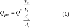
Here Q is the observed volume (in vehicles per hour), vi and Ai are the average spot speed and plan area of the ith category vehicle and vc and Ac are the corresponding spot speed and plan area of cars. The Table 4 was referred for the values of plan area of different vehicle categories.

Spot speeds obtained by radar gun were averaged over
the count period and then were converted to stream speed, the speed with
which the average vehicle moves on that spot, equivalent to the PCU of
traffic volume, using the following formula:
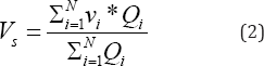
Here, Vs is the stream speed, vi is the average spot speed and Qi the volume (vehicles per hour) of the ith category vehicle and N is the number of categories (=6).
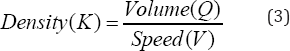
The computed values of stream volume and speed at
nodes were used to calculate the traffic density of the sections.
Density is a traffic flow parameter that depicts the "crowdedness" of
the traffic stream, an important indicator of congestion used especially
in capacity based quantification of congestion:
Finally, the estimated average values of the traffic
volume, speed and density across segments were computed by simply
averaging the values of the origin and destination nodes.
Modelling
Selection of variables
The primary aim of this study being
origin-destination based congestion estimation, different node variables
were tested for correlation both among themselves as well as with the
dependent variable Travel Time. In the Pearson correlation matrix of the
independent variables, all but five correlation coefficients came out
to be between -0.5 and 0.5, leading to the conclusion that most of them
are really independent. Also, all but two variables, viz. 'Number of
Lanes' and 'Destination Speed', were found to be reasonably related to
the dependent variable, with their correlation coefficients greater than
0.5. The values are tabulated in Table 5.

Model development
With the given data, two datasets were created: one
with the source-destination values, the other one with segment values
averaged from the first set.
Both linear and exponential multivariate models were
developed for each of the two datasets with the help of IBM SPSS, a
statistical analysis software application. Analysis of Variance (ANOVA)
was carried out on the four models. F test was carried out on the models
with a DDF (denominator degrees of freedom) of 383 on a confidence
interval of 95%. The results are given in the Table 6

Thus Model 1, which has the highest R2
value and the best F value, was chosen as the desired model. The
following formula of travel time (in seconds) was arrived at. The
symbols denote the variables as mentioned in Table 5.
On putting the values of all parameters in equation 6
for all the segments, the value obtained for travel time during morning
peak and evening peak hours are given in Table 7.
Model 1:
T= -94. 1+15 . 2*L +135 . 6*N,+0 . 27*Qs0 . 15*ft -23 . 9*V +26.0*^-6. 16* K + 4. 89%

Validation of model
Modelling by regression was carried out with 75% of
the pre-processed data, while the remaining 25% was used for validation
of the same model. This was done by finding out Normalized Root Mean
Squared Error (NRMSE) and Mean Absolute Percentage Error (MAPE), values
that determine the predictive power of the model. They are given by the
following formulae: -
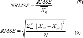
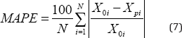
Here Xo is the actual value of the parameter, Xp is
its predicted value according to the model, is the mean of the observed
values and N is the total number of observations in the validation
dataset. A low value of these values is desirable; typically, a value of
around 0.1 (10%) of NRMSE and MAPE depict a highly accurate model. The
obtained values on the validation dataset in this linear
source-destination (Model 1) model are given in Table 8. The values of NRMSE and MAPE imply a substantially accurate forecasting. From the Predicted Time vs. Observed Time graph in Figure 1, it may be understood that the applied model works well for the validation dataset.


Free Flow and Congestion
The finalized model gives an estimate of the travel
time in each trip on a given segment, but it does not conclusively
depict the state of congestion on the segment. The average value of
Congestion Index (CI) in the peak hour was calculated for each segment
with the help of the following formula: -
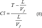
Where T is the average of the travel times, L is the
segment length and Vf is taken as 55kmph.The CI values obtained for the
morning and evening peak hours and level of congestion in the study
route is shown in Table 9.
The priority values obtained for the different segments in the study route on the basis of congestion level is shown in Table 10.
The priority values obtained in ascending order imply that segment 2
and 3 (i.e., Sarai Kale Khan to Andrew Ganj to AIIMS North) with
priority number 1 remain extremely congested especially during the
evening peak time, with as high an average value of 2.71 implying that
an about 8 1/2 minutes long commute at midnight usually takes about 29
minutes during the evening.


The obtained values of congestion index are
significantly higher than typical values of cities as a whole, as
suggested by TomTom, which classifies cities with CI values above 0.5 as
reasonably congested. This is partly attributed to the nature of the
study with specific focus on busy arterials instead of the entire road
network that in general faces a lesser degree of congestion. However,
with this study it is clearly established that the south-eastern portion
of the Inner Ring Road of Delhi (study segments 2 and 3 with priority
number 1 becomes extraordinarily congested at peak times and thus needs
to be immediately checked for congestion reduction measures.
Conclusion
This paper proposes an idea of estimating congestion
on urban roads with reduced cost of field data collection by limiting
observation sites at only a few select points (nodes) in the route
instead of the entire length. A model for prediction of travel time on a
given segment was prepared using multiple linear regressions. Combined
with the knowledge of free flow time for that segment, which from among
other methods can also be approximated from the midnight field
observation data, Congestion Index, which is an efficient, route length
independent measure of congestion, can be calculated. This procedure was
carried out in this study for a major road route in Delhi. Data for
travel times by a bus and category wise spot speed and volume were
collected, analyzed and used for modeling, as well as for validation of
the same model. Different combinations of situations were analyzed to
arrive at four efficient models, of which one with the best statistical
values was chosen (adjusted R2=0.917). The model was validated with the
help of root mean squared error (RMSE) evaluation, which with a value of
7.2% was found remarkably reliable.
It can also be seen that this study, due to the
virtue of scope, has some limitations that were duly noted. The use of
node data to estimate travel time may help in estimation of travel time,
but it falters in providing help for suggesting alternative routes
because the node data for alternative routes remain the same
notwithstanding anything but roadway parameters such as length and
diversions. In order to make this distinction clear, more roadway
parameters should be studied for influence on traffic congestion.
For More Open Access Journals Please Click on: Juniper Publishers
Fore More Articles Please Visit: Civil Engineering Research Journal
Fore More Articles Please Visit: Civil Engineering Research Journal


Comments
Post a Comment